1 Introduction to Coordinate Frames and Reference Points
1.1 Introduction
This first lecture introduces the fundamental concepts needed to describe the motion of marine vehicles. The analysis and control of ships, submarines, and other marine craft requires a mathematical framework for representing their position, orientation, and velocities. This necessitates defining appropriate coordinate systems and notation conventions.
After this lecture students should be able to:
- Understand the coordinate frames used in marine vehicle dynamics
- Identify the reference points on a marine vehicle
- Use vector notation to describe position, orientation, and velocity vectors
- Define generalized coordinates for marine vehicles
1.2 Coordinate Frames
The definition of velocities, positions, and orientations of a marine vehicle requires establishing appropriate coordinate frames. Two main types of coordinate frames can be distinguished as:
- Inertial frames: These are fixed relative to the Earth. Newton’s laws apply in these frames.
- Non-inertial frames: These are accelerating relative to the Earth. Newton’s laws do not apply in these frames.
The important frames of reference for studying the motion of marine vehicles are:
- Earth-Centered Inertial (ECI) Frame
- Earth-Centered Earth-Fixed (ECEF) Frame
- North-East-Down (NED) Frame
- Body-Fixed Frame
1.2.1 Earth-Centered Inertial (ECI) Frame
The Earth-centered inertial (ECI) frame, denoted \(\{i\}\), is defined as:
\[\begin{align} \{i\} = (x^i, y^i, z^i) \end{align}\]
- Origin \(O_i\) is at the center of the Earth with z-axis going through the axis of rotation of the Earth
- Non-accelerating reference frame where Newton’s laws apply
- Used in designing inertial navigation systems and terrestrial navigation
1.2.2 Earth-Centered Earth-Fixed (ECEF) Frame
The Earth-centered Earth-fixed (ECEF) frame, denoted \(\{e\}\), is defined as:
\[\begin{align} \{e\} = (x^e, y^e, z^e) \end{align}\]
- Origin \(O_e\) is at the center of the Earth
- Rotates relative to the ECI frame
- \(x_e\) axis points to the prime meridian in the equatorial plane
- \(y_e\) axis completes the right-handed system in the equatorial plane
- \(z_e\) axis points along Earth’s rotational axis
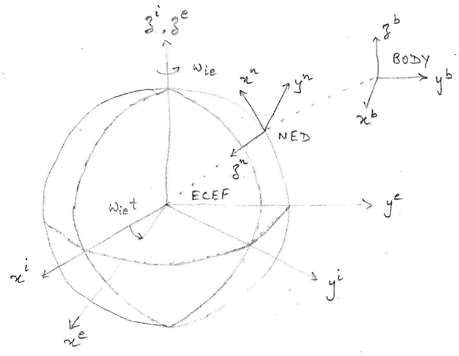
The Earth’s rotation rate is:
\[\omega_{ie} = \frac{2\pi}{24 \times 60 \times 60} = 7.2921 \times 10^{-5} \text{ rad/s}\]
The Earth’s rotational vector in the ECEF frame is:
\[\omega_{ie}^e = \vec{\omega}_{ie}^e = \{\omega_{ie}^e\} = [0 \quad 0 \quad \omega_{ie}]^T\]
The ECEF frame is used for global navigation applications.
1.2.3 North-East-Down (NED) Frame
The North-East-Down (NED) frame, denoted \(\{n\}\), is defined as:
\[\begin{align} \{n\} = (x^n, y^n, z^n) \end{align}\]
- Origin \(O_n\) is defined as the location where the tangent plane touches the Earth’s reference ellipsoid (World Geodetic System 1984 - WGS84)
- Used for local navigation (valid over approximately 10 km x 10 km area)
- x-axis points North
- y-axis points East
- z-axis points Down
The location of the NED frame relative to the ECEF frame is determined using two angles:
- \(l\) : longitude
- \(\mu\) : latitude
1.2.4 Body-Fixed Frame
The body-fixed coordinate frame, denoted by \(\{b\}\), is defined as:
\[\begin{align} \{b\} = (x^b, y^b, z^b) \end{align}\]
- Origin \(O_b\) is chosen at a convenient point on the vessel
- Typically at the intersection of the midship waterline and centerline
- \(x^b\) axis points from aft to fore
- \(y^b\) axis points to starboard
- \(z^b\) axis points from top to bottom
1.3 Reference Points
Several key reference points are defined on a marine vehicle:
CO: Coordinate origin \(O_b\) - origin of the body-fixed frame {b}
CG: Center of gravity relative to \(O_b\) \[\begin{align} \vec{r}_{bg}^b = \{r_{bg}^b\} = [x_g \quad y_g \quad z_g]^T \end{align}\]
CB: Center of buoyancy relative to \(O_b\) \[\begin{align} \vec{r}_{bb}^b = \{r_{bb}^b\} = [x_b \quad y_b \quad z_b]^T \end{align}\]
CF: Center of flotation relative to \(O_b\) \[\begin{align} \vec{r}_{bf}^b = \{r_{bf}^b\} = [x_f \quad y_f \quad z_f]^T \end{align}\] This is the centroid of the waterplane area.
The coordinate origin CO has a constant location, while CG, CB, and CF can vary with time depending on loading conditions, ballast levels, weather, and vehicle motions.
1.4 Generalized Coordinates
Generalized coordinates are parameters that describe the configuration of the marine vehicle relative to a reference configuration.
1.4.1 Generalized Position
The generalized position vector \(\{\eta\}\) is defined as:
\[\begin{align} \{\eta\} = [x^n \quad y^n \quad z^n \quad \phi \quad \theta \quad \psi]^T \in \mathbb{R}^6 \end{align}\]
where:
- \((x^n, y^n, z^n)\) is the position of CO in the NED frame
- \((\phi, \theta, \psi)\) are the Euler angles representing the orientation of the body-fixed frame relative to the NED frame
1.4.2 Generalized Velocity
The generalized velocity vector \(\{v\}\) in the body-fixed frame is defined as:
\[\begin{align} \{v\} = [u \quad v \quad w \quad p \quad q \quad r]^T \in \mathbb{R}^6 \end{align}\]
where:
- \((u, v, w)\) are the linear velocity components in the body-fixed frame
- \((p, q, r)\) are the angular velocity components in the body-fixed frame
1.5 Vector Notation
Two notations are used to represent vectors in 3D space:
Vector notation: \[\begin{align} \vec{a} = a_1^n \hat{n}_1 + a_2^n \hat{n}_2 + a_3^n \hat{n}_3 \end{align}\] where \(\hat{n}_1, \hat{n}_2, \hat{n}_3\) are unit vectors along the \(x^n, y^n, z^n\) axes.
Coordinate form: \[\begin{align} \{a^n\} = [a_1^n \quad a_2^n \quad a_3^n]^T \in \mathbb{R}^3 \end{align}\]
Both notations are used interchangeably in this course.
1.6 Key Vector Definitions
The following vectors are defined for a marine vehicle:
- \(\{p_{eb}^e\}\): Position of CO relative to \(O_e\) expressed in {e}
- \(\{p_{nb}^n\}\): Position of CO relative to \(O_n\) expressed in {n}
- \(\{v_{nb}^b\}\): Linear velocity of CO relative to \(O_n\) expressed in {b}
- \(\{\omega_{nb}^b\}\): Angular velocity of \(\{b\}\) relative to \(\{n\}\) expressed in \(\{b\}\)
- \(\{f_b^b\}\): Force with line of action through CO expressed in \(\{b\}\)
- \(\{m_b^b\}\): Moment about CO expressed in \(\{b\}\)
- \(\{\Theta_{nb}\}\): Euler angles from \(\{n\}\) to \(\{b\}\)
- \(\{\Theta_{en}\}\): Longitude and latitude
These vectors are expressed as:
\[\begin{align} \{p_{eb}^e\} &= [x^e \quad y^e \quad z^e]^T \in \mathbb{R}^3 \quad \text{(ECEF position)} \\ \{p_{nb}^n\} &= [x^n \quad y^n \quad z^n]^T \in \mathbb{R}^3 \quad \text{(NED position)} \\ \{v_{nb}^b\} &= [u \quad v \quad w]^T \in \mathbb{R}^3 \quad \text{(Body-fixed linear velocity)} \\ \{f_b^b\} &= [X \quad Y \quad Z]^T \in \mathbb{R}^3 \quad \text{(Body-fixed force)} \\ \{m_b^b\} &= [K \quad M \quad N]^T \in \mathbb{R}^3 \quad \text{(Body-fixed moment)} \\ \{\omega_{nb}^b\} &= [p \quad q \quad r]^T \in \mathbb{R}^3 \quad \text{(Body-fixed angular velocity)} \\ \{\Theta_{nb}\} &= [\phi \quad \theta \quad \psi]^T \in \Pi^3 \quad \text{(Euler angles)} \\ \{\Theta_{en}\} &= [l \quad \mu]^T \in \Pi^2 \quad \text{(Longitude and latitude)} \end{align}\]
The generalized position, velocity, and force vectors are defined as:
\[\begin{align} \{\eta\} &= \begin{bmatrix} p_{nb}^n \\ \Theta_{nb} \end{bmatrix} \\ \{\nu\} &= \begin{bmatrix} v_{nb}^b \\ \omega_{nb}^b \end{bmatrix} \\ \{\tau\} &= \begin{bmatrix} f_b^b \\ m_b^b \end{bmatrix} \end{align}\]
where:
\[\begin{align} \{\eta\} \in \mathbb{R}^3 \times \Pi^3, \quad \{\nu\} \in \mathbb{R}^6, \quad \{\tau\} \in \mathbb{R}^6 \end{align}\]
and \(\Pi^3 = \mathbb{S}^1 \times \mathbb{S}^1 \times \mathbb{S}^1 \subset \mathbb{R}^3\) is the 3D torus.
Each Euler angle is defined in the range \([-\pi, \pi)\).