2  Coordinate Transformations and Kinematics with Euler Angles

2.1 Introduction to Coordinate Transformations

This lecture focuses on coordinate transformations and kinematics. The lecture explores how to represent and transform coordinates between different reference frames, with a particular emphasis on transformations between body-fixed and inertial (NED - North-East-Down) coordinate systems.

After this lecture students should be able to:

• Understand the coordinate transformations between different reference frames
• Use rotation matrices to transform vectors between different coordinate frames
• Relate angular velocities to the Euler angle rates and vice versa
• Derive the kinematic equations for a marine vehicle

2.2 Rotation Matrices

Rotation matrices are fundamental to coordinate transformations. A rotation matrix between two frames \(\{a\}\) and \(\{b\}\) is denoted as \([R_b^a]\). Rotation matrices are elements of the Special Orthogonal Group of order 3, denoted as SO(3), which is defined as:

\[\begin{align} \text{SO(3)} \subset \text{O(3)} := \{[R]: [R] \in \mathbb{R}^{3\times3}, [R][R]^T = [R]^T[R] = [I_3]\} \end{align}\]

The convention for naming rotation matrices is shown below:

\[\begin{align} \{v^a\} = [R_b^a]\{v^b\} \end{align}\]

where \(\{v^a\}\) is a vector expressed in frame \(\{a\}\), \(\{v^b\}\) is the same vector expressed in frame \(\{b\}\), and \([R_b^a]\) is the rotation matrix that transforms a vector from frame \(\{b\}\) to frame \(\{a\}\). Because of the orthogonality property, the rotation matrix for transforming a vector from frame \(\{a\}\) to frame \(\{b\}\) is given by \([R_a^b] = [R_b^a]^{-1} = [R_b^a]^T\).

2.3 Skew-Symmetric Matrices

Skew-symmetric matrices are useful in representing cross products as matrix multiplications. A skew-symmetric matrix \([S]\) has the property \([S] = -[S]^T\).

For a vector \(\vec{\lambda}\), the cross product \(\vec{\lambda} \times \vec{a}\) can be represented as a matrix multiplication:

\[\begin{align} \vec{\lambda} \times \vec{a} := [S(\lambda)]\{a\} \end{align}\]

where:

\[\begin{align} [S(\lambda)] = -[S(\lambda)]^T = \begin{bmatrix} 0 & -\lambda_3 & \lambda_2 \\ \lambda_3 & 0 & -\lambda_1 \\ -\lambda_2 & \lambda_1 & 0 \end{bmatrix} \end{align}\]

2.4 Transformations between Body and NED Frames

Just as translations in 3D space can be described by three components \((x^n, y^n, z^n)\), rotations can also be described by three components \((\phi, \theta, \psi)\). These three angles that describe the orientation of a rigid body are called Euler angles. However, unlike translations which are commutative (the order doesn’t matter), rotations are non-commutative. This means that the final orientation depends on the sequence in which the rotations are performed.

Euler angles provide an intuitive way to describe the orientation of a rigid body by decomposing the complete rotation into three sequential rotations about different axes. While there are twelve possible sequences of rotations (like XYZ, ZYX, ZXY, etc.), in marine vehicles we typically use the ZYX convention, also known as the yaw-pitch-roll sequence.

The transformation from the NED frame to the body-fixed frame follows this sequence:

1. First rotation about the z-axis by angle \(\psi\) (yaw) - this represents the heading or yaw angle
2. Second rotation about the new y-axis by angle \(\theta\) (pitch) - this represents the pitch angle
3. Final rotation about the new x-axis by angle \(\phi\) (roll) - this represents the roll angle

Let’s define the intermediate frames through which the rotation happens:

1. Frame 3, denoted as \(\{3\}\), represents the coordinate frame after translation but before any rotation is applied. This frame has its origin at the body-fixed point \(O_b\), but its axes remain parallel to those of the NED frame since no rotation has occurred yet. Frame 3 serves as the initial reference frame from which we will begin applying our sequence of rotations.

2. Frame 2, denoted as \(\{2\}\), is obtained by rotating the frame \(\{3\}\) about its z-axis by angle \(\psi\). This first rotation is represented by the transformation matrix \([R_{z,\psi}]\) which maps vectors from frame \(\{3\}\) to frame \(\{2\}\).

3. Frame 1, denoted as \(\{1\}\), is obtained by rotating frame \(\{2\}\) about its y-axis by angle \(\theta\). This second rotation is represented by the transformation matrix \([R_{y,\theta}]\) which maps vectors from frame \(\{2\}\) to frame \(\{1\}\).

4. Body fixed frame, denoted as \(\{b\}\), is obtained by rotating frame \(\{1\}\) about its x-axis by angle \(\phi\). This final rotation is represented by the transformation matrix \([R_{x,\phi}]\) which maps vectors from frame \(\{1\}\) to frame \(\{b\}\).

Therefore, the complete transformation from NED to body-fixed frame can be written as a sequence:

\[\begin{align} \{n\} \xrightarrow{\text{translate}(x^n,y^n,z^n)} \{3\} \xrightarrow{[R_{z,\psi}]} \{2\} \xrightarrow{[R_{y,\theta}]} \{1\} \xrightarrow{[R_{x,\phi}]} \{0\} \nonumber \end{align}\]

The rotation matrices for each step are:

1. Rotation about z-axis (yaw):

   From Figure 2.1 it can be seen that the z-axis is pointed into the page and the positive direction of \(\psi\) is counterclockwise. Note that z-coordinates remain unchanged since rotation is about z-axis. Assuming that the velocity vector of the vessel is denoted by \(\vec{v}_{nb}^{n} = \vec{v}_{nb}^{3} = \vec{U} = [u_3, v_3, w_3]^T\), the velocity vector in frame \(\{3\}\) can be expressed in terms of velocity expressed in frame \(\{2\}\) \(\vec{v}_{nb}^{2} = [u_2, v_2, w_2]^T\) as:

   \[\begin{align} \{v_{nb}^3\} = [R_{z,\psi}]\{v_{nb}^2\} \end{align}\]

   \[\begin{align} \begin{bmatrix} u_3 \\ v_3 \\ w_3 \end{bmatrix} = \begin{bmatrix} \cos(\psi) & -\sin(\psi) & 0 \\ \sin(\psi) & \cos(\psi) & 0 \\ 0 & 0 & 1 \end{bmatrix} \begin{bmatrix} u_2 \\ v_2 \\ w_2 \end{bmatrix} \end{align}\]

   where:

   \[\begin{align} [R_{z,\psi}] = \begin{bmatrix} \cos(\psi) & -\sin(\psi) & 0 \\ \sin(\psi) & \cos(\psi) & 0 \\ 0 & 0 & 1 \end{bmatrix} \end{align}\]

   

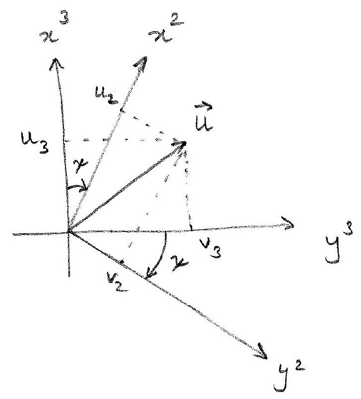
   Figure 2.1: Yaw rotation

2. Rotation about y-axis (pitch):

   From Figure 2.2 it can be seen that the y-axis is pointed into the page and the positive direction of \(\theta\) is counterclockwise. Note that y-coordinates remain unchanged since rotation is about y-axis. The velocity vector in frame \(\{2\}\) \(\vec{v}_{nb}^{2} = [u_2, v_2, w_2]^T\) can be expressed in terms of velocity expressed in frame \(\{1\}\) \(\vec{v}_{nb}^{1} = [u_1, v_1, w_1]^T\) as:

   \[\begin{align} \{v_{nb}^2\} = [R_{y,\theta}]\{v_{nb}^1\} \end{align}\]

   \[\begin{align} \begin{bmatrix} u_2 \\ v_2 \\ w_2 \end{bmatrix} = \begin{bmatrix} \cos(\theta) & 0 & \sin(\theta) \\ 0 & 1 & 0 \\ -\sin(\theta) & 0 & \cos(\theta) \end{bmatrix} \begin{bmatrix} u_1 \\ v_1 \\ w_1 \end{bmatrix} \end{align}\]

   where:

   \[\begin{align} [R_{y,\theta}] = \begin{bmatrix} \cos(\theta) & 0 & \sin(\theta) \\ 0 & 1 & 0 \\ -\sin(\theta) & 0 & \cos(\theta) \end{bmatrix} \end{align}\]

   

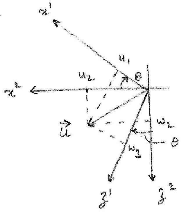
   Figure 2.2: Pitch rotation

3. Rotation about x-axis (roll):

   From Figure 2.3 it can be seen that the x-axis is pointed into the page and the positive direction of \(\phi\) is counterclockwise. Note that x-coordinates remain unchanged since rotation is about x-axis. The velocity vector in frame \(\{1\}\) \(\vec{v}_{nb}^{1} = [u_1, v_1, w_1]^T\) can be expressed in terms of velocity expressed in frame \(\{b\}\) \(\vec{v}_{nb}^{b} = [u, v, w]^T\) as:

   \[\begin{align} \{v_{nb}^1\} = [R_{x,\phi}]\{v_{nb}^b\} \end{align}\]

   \[\begin{align} \begin{bmatrix} u_1 \\ v_1 \\ w_1 \end{bmatrix} = \begin{bmatrix} 1 & 0 & 0 \\ 0 & \cos(\phi) & -\sin(\phi) \\ 0 & \sin(\phi) & \cos(\phi) \end{bmatrix} \begin{bmatrix} u \\ v \\ w \end{bmatrix} \end{align}\]

   where:

   \[\begin{align} [R_{x,\phi}] = \begin{bmatrix} 1 & 0 & 0 \\ 0 & \cos(\phi) & -\sin(\phi) \\ 0 & \sin(\phi) & \cos(\phi) \end{bmatrix} \end{align}\]

   

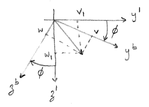
   Figure 2.3: Roll rotation

The complete rotation matrix from the body-fixed frame to the NED frame is:

\[\begin{align} [R_b^n] = [R_{z,\psi}][R_{y,\theta}][R_{x,\phi}] \end{align}\]

The full rotation matrix is:

\[\begin{align} [R_b^n] = \begin{bmatrix} c_{\psi}c_{\theta} & -s_{\psi}c_{\phi} + c_{\psi}s_{\theta}s_{\phi} & s_{\psi}s_{\phi} + c_{\psi}s_{\theta}c_{\phi} \\ s_{\psi}c_{\theta} & c_{\psi}c_{\phi} + s_{\psi}s_{\theta}s_{\phi} & -c_{\psi}s_{\phi} + s_{\psi}s_{\theta}c_{\phi} \\ -s_{\theta} & c_{\theta}s_{\phi} & c_{\theta}c_{\phi} \end{bmatrix} \end{align}\]

where \(c_{\psi} = \cos(\psi), s_{\psi} = \sin(\psi), c_{\theta} = \cos(\theta), s_{\theta} = \sin(\theta), c_{\phi} = \cos(\phi), s_{\phi} = \sin(\phi)\). For small angles \(\delta\phi, \delta\theta, \delta\psi\), this can be approximated as:

\[\begin{align} [R_b^n] \approx \begin{bmatrix} 1 & -\delta\psi & \delta\theta \\ \delta\psi & 1 & -\delta\phi \\ -\delta\theta & \delta\phi & 1 \end{bmatrix} = [I_3] + [S(\delta\Theta_{nb})] \end{align}\]

2.5 Velocity Transformations

The body-fixed velocity vector \(\{v_{nb}^b\}\) can be expressed in the NED frame as:

\[\begin{align} \{\dot{p}_{nb}^n\} = \{v_{nb}^n\} = [R_b^n]\{v_{nb}^b\} = [R(\Theta_{nb})]\{v_{nb}^b\} \end{align}\]

Similarly, the NED frame velocity can be expressed in the body-fixed frame:

\[\begin{align} \{v_{nb}^b\} = [R^{-1}(\Theta_{nb})]\{\dot{p}_{nb}^n\} = [R(\Theta_{nb})]^T\{\dot{p}_{nb}^n\} \end{align}\]

2.6 Gimbal Lock

It can be seen that when \(\theta = \frac{\pi}{2}\) the rotation matrix \([R_b^n]\) reduces to as shown in \(\eqref{eq-rotm-gimbal-lock}\).

\[\begin{align} [R_b^n] &= \begin{bmatrix} 0 & -c_{\phi}s_{\phi} + s_{\phi}c_{\psi} & s_{\phi}s_{\psi} + c_{\phi}c_{\psi} \\ 0 & c_{\phi}c_{\psi} + s_{\phi}s_{\psi} & c_{\phi}s_{\psi} - s_{\phi}c_{\psi} \\ -1 & 0 & 0 \end{bmatrix} \nonumber \\ &= \begin{bmatrix} 0 & \sin(\phi - \psi) & \cos(\phi - \psi) \\ 0 & \cos(\phi - \psi) & -\sin(\phi - \psi) \\ -1 & 0 & 0 \end{bmatrix} \label{eq-rotm-gimbal-lock} \end{align}\]

In this case the rotation matrix becomes degenerate. This means that unique mapping is lost at this point. Several combinations of \(\phi\) and \(\psi\) that have the same value of \(\phi - \psi\) will lead to the same rotation matrix. For example, \((\phi, \theta, \psi) = (10^\circ, 90^\circ, 5^\circ)\) and \((\phi, \theta, \psi) = (5^\circ, 90^\circ, 0^\circ)\) will lead to the same rotation matrix. This phenomenon is called gimbal lock. It is called a gimbal lock as in this representation there is no way to roll the vehicle (for the ZYX rotation order) without pitching it out of the gimbal lock position.

For Euler angle formulation based on ZYX order of rotation, gimbal lock will happen when \(\theta = \frac{n\pi}{2}\) for \(n=\pm1, \pm2, ...\) Note that this phenomenon happens for all Euler angle formulations regardless of the order of rotation. Whenever the second rotation results in the first and the third axes of rotations being coincident, this degeneracy will manifest.

Common Confusion

The common confusion is - does physically the rigid body experience any problem when passing through this degenerate point of \(\theta = \pm \frac{\pi}{2}\)?

Remember that the Euler angle notation is our way of representing the pose of the rigid body. The degenracy is in our way of representing the orientation and not with the physical world. So when physically the rigid body moves through a gimbal lock orientation, our representation of orientation will result in a funny looking motion. Quaternions based representation of oreintation does not suffer from the problem of gimbal lock and hence has been widely adopted in the fields of robotics, computer vision, computer graphics, flight dynamics etc.

Check out this YouTube video on Gimbal lock for better visualization.

There exist 12 different possible rotation orders when defining Euler angles. These can be separated into two groups:

• Proper Euler Angles (ZXZ, XYX, YZY, ZYZ, XZX and YXY)
• Tait-Bryan Angles (XYZ, ZXY, YZX, XZY, ZYX and YZX)

The Tait-Bryan angles represent rotations about three distinct axes while proper Euler angles use the same axes for the first and third elemental rotations. For marine vehicles, the common rotation order used is ZYX order. Notice that for this choice of rotation order, the gimbal lock orientations occur when the vehicle pitches up or down by \(90^{\circ}\). As marine vehicles like ships and underwater vehicles do not pitch by large angles during regular operations, this representation serves well to describe orientations uniquely. Unless specified explicitly, this text will assume a ZYX order of rotation when referring to Euler angles.

2.7 Angular Velocity Transformation

The angular velocity transformation is given by:

\[\begin{align} \{\omega_{nb}^b\} &= \begin{bmatrix} \dot{\phi} \\ 0 \\ 0 \end{bmatrix} + [R_{x,\phi}]^T \begin{bmatrix} 0 \\ \dot{\theta} \\ 0 \end{bmatrix} + [R_{x,\phi}]^T [R_{y,\theta}]^T \begin{bmatrix} 0 \\ 0 \\ \dot{\psi} \end{bmatrix} \\ &= \begin{bmatrix} 1 & 0 & -s_{\theta} \\ 0 & c_{\phi} & c_{\theta}s_{\phi} \\ 0 & -s_{\phi} & c_{\theta}c_{\phi} \end{bmatrix} \begin{bmatrix} \dot{\phi} \\ \dot{\theta} \\ \dot{\psi} \end{bmatrix} \\ &= [T^{-1}(\Theta_{nb})]\{ \dot{\Theta}_{nb} \} \end{align}\]

where

\[\begin{align} [T(\Theta_{nb})] &= \begin{bmatrix} 1 & s_{\phi}t_{\theta} & c_{\phi}t_{\theta} \\ 0 & c_{\phi} & -s_{\phi} \\ 0 & s_{\phi}/c_{\theta} & c_{\phi}/c_{\theta} \end{bmatrix} \end{align}\]

where \(t_{\theta} = \tan(\theta)\).For small angles \(\delta\phi, \delta\theta, \delta\psi\), this can be approximated as:

\[\begin{align} [T(\delta\Theta_{nb})] = \begin{bmatrix} 1 & 0 & \delta\theta \\ 0 & 1 & -\delta\phi \\ 0 & \delta\phi & 1 \end{bmatrix} \end{align}\]

2.8 Rotation Matrix Differential Equation

It can be shown that the differential equation for the rotation matrix is:

\[\begin{align} [\dot{R}_b^n] = [R_b^n][S(\omega_{nb}^b)] \end{align}\]

where:

\[\begin{align} [S(\omega_{nb}^b)] = \begin{bmatrix} 0 & -r & q \\ r & 0 & -p \\ -q & p & 0 \end{bmatrix} \end{align}\]

2.9 6-DOF Kinematic Equations

The 6DOF kinematic equations can be expressed as:

\[\begin{align} \{\dot{\eta}\} &= [J_0(\eta)]\{v\} \\ \begin{bmatrix} \dot{p}_{nb}^n \\ \dot{\Theta}_{nb} \end{bmatrix} &= \begin{bmatrix} R(\Theta_{nb}) & 0_{3\times3} \\ 0_{3\times3} & T(\Theta_{nb}) \end{bmatrix} \begin{bmatrix} v_{nb}^b \\ \omega_{nb}^b \end{bmatrix} \end{align}\]

where \(\{\eta\} \in \mathbb{R}^3 \times \mathbb{T}^3, \{v\} \in \mathbb{R}^6\).

2.10 3-DOF Kinematic Equations

For horizontal modes (surge, sway, and yaw), assuming small roll and pitch angles during normal operation, the equations can be simplified:

\[\begin{align} [R(\Theta_{nb})] &= [R_{z,\psi}][R_{y,\theta}][R_{x,\phi}] \approx [R_{z,\psi}] \\ [T(\Theta_{nb})] &\approx [I_3] \end{align}\]

In this case:

\[\begin{align} \{\dot{\eta}\} &= [R(\psi)]\{v\} \end{align}\]

where \([R(\psi)] := [R_{z,\psi}]\), \(\{v\} = [u, v, r]^T\) and \(\{\eta\} = [x^n, y^n, \psi]^T\). These equations provide a simplified model for planar motion, which is often sufficient for many marine robotic applications involving surface vessels.